← All four projectsProject notes

TinyML

Voice commands on a small board, with questions about audio, classification, timing and energy.

NOTE
TinyML

A prediction is the end of the route, not the whole project

The voice project ends each processing pass with OFF, ON or noise, but the prediction is only the last visible part of the route. The export expects 16,000 raw samples at 16 kHz and uses a 650-value feature representation for three classes. The application has to supply that input before the mo

·4 min read
NOTE
TinyML

What the battery would have to power between predictions

The classifier is only one part of what a battery would power. The application collects a complete audio frame, processes it, prints timings and class probabilities, then waits for one second. The code's delay does not put the controller into a documented sleep mode, and the application does no

·4 min read
NOTE
TinyML

I can calculate 46.3 millijoules. What did those millijoules do?

I recorded 14.04 mC at a 3.3 V supply over a 257.8 ms inference window. Multiplying the charge by the supply voltage gave 46.332 mJ, or about 46.3 mJ per inference. I checked the calculation against the average current and duration before writing the result down.

·4 min read
NOTE
TinyML

The code has started drawing a current graph

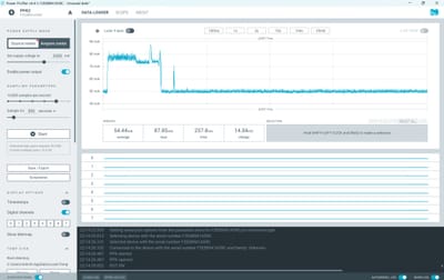
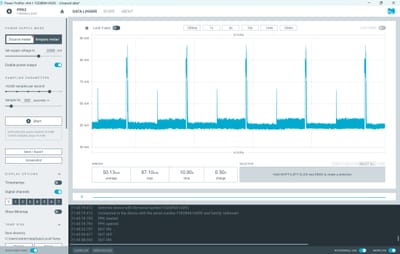
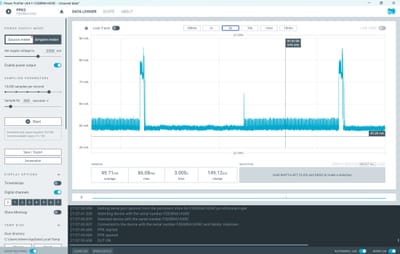
The PPK2 views show two different electrical windows at a 3.3 V source setting. The wider view covers 10 seconds, with 50.13 mA average current, 87.10 mA maximum and 0.50 C of charge. The closer view covers 257.8 ms, with 54.44 mA average, 87.85 mA maximum and 14.04 mC. The time boundary is par

·4 min read
NOTE
TinyML

Why does the model look better on the screen than through the microphone?

The live microphone results were less encouraging than the validation screen. That made the route into the classifier more interesting to me. A model file does not receive the word ON as a meaning; it receives a representation of the captured sound. The laptop recordings and the INMP441 stream

·5 min read
NOTE
TinyML

Three milliseconds sounded great, until I read the target name

I timed the classifier on the ESP32-S3: 3 ms for INT8 and 35 ms for floating point. Three milliseconds felt quick, but the feature-processing stage still needed attention. I kept its timing separate from the classifier so I could see where the complete processing pass spent its time.

·4 min read
NOTE
TinyML

The big percentage was not the most interesting thing on the screen

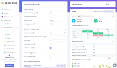
The validation screen gives 88.2% accuracy and a loss of 0.28. The confusion matrix makes the result more particular: the OFF and ON rows are in their correct columns, while the noise row is split equally between ON and noise. That’s the part I want to understand before treating the overall per

·4 min read
NOTE
TinyML

Trying to understand the part between the sound and the model

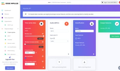
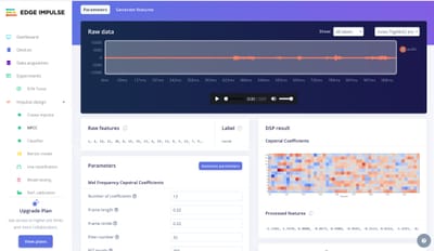
The MFCC block has definite settings: 13 cepstral coefficients, 20 ms frames, a 20 ms stride, 32 filters and a 256-point FFT. Its output is a 650-value feature representation, while the audio window begins with 16,000 raw samples at 16 kHz. Those are different stages of the route from sound to

·4 min read
NOTE
TinyML

A hundred recordings become one minute and forty seconds

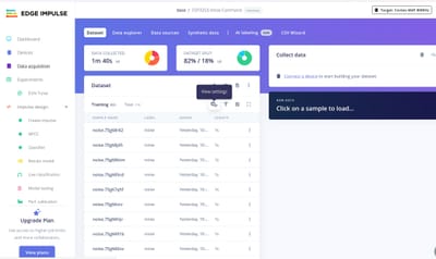
The dataset view contains 100 one-second clips: one minute and forty seconds of sound. The split is 82 training examples and 18 test examples. That’s a concrete scale I can think about, rather than simply calling the dataset small or large. Each second is one of the examples behind the patterns

·4 min read
NOTE
TinyML

Before I blame the model, what did the microphone send it?

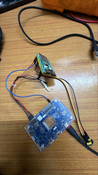
The microphone test has a smaller job than the classifier. Its code sets 16 kHz, 32-bit left-channel I²S, with word select on GPIO 15, data on 16 and clock on 14. It reads blocks into an int32 buffer, then prints a value called SoundLevel. Before treating that number as evidence about a word, I

·3 min read
NOTE
TinyML

Two short words, and everything the microphone hears around them

OFF, ON and noise are the three classes in the exported voice model. The application begins with a one-second audio window: 16,000 raw samples at 16 kHz. After feature processing, the model has a 650-value input and produces predictions for those three labels. That’s a much more interesting rou

·4 min read