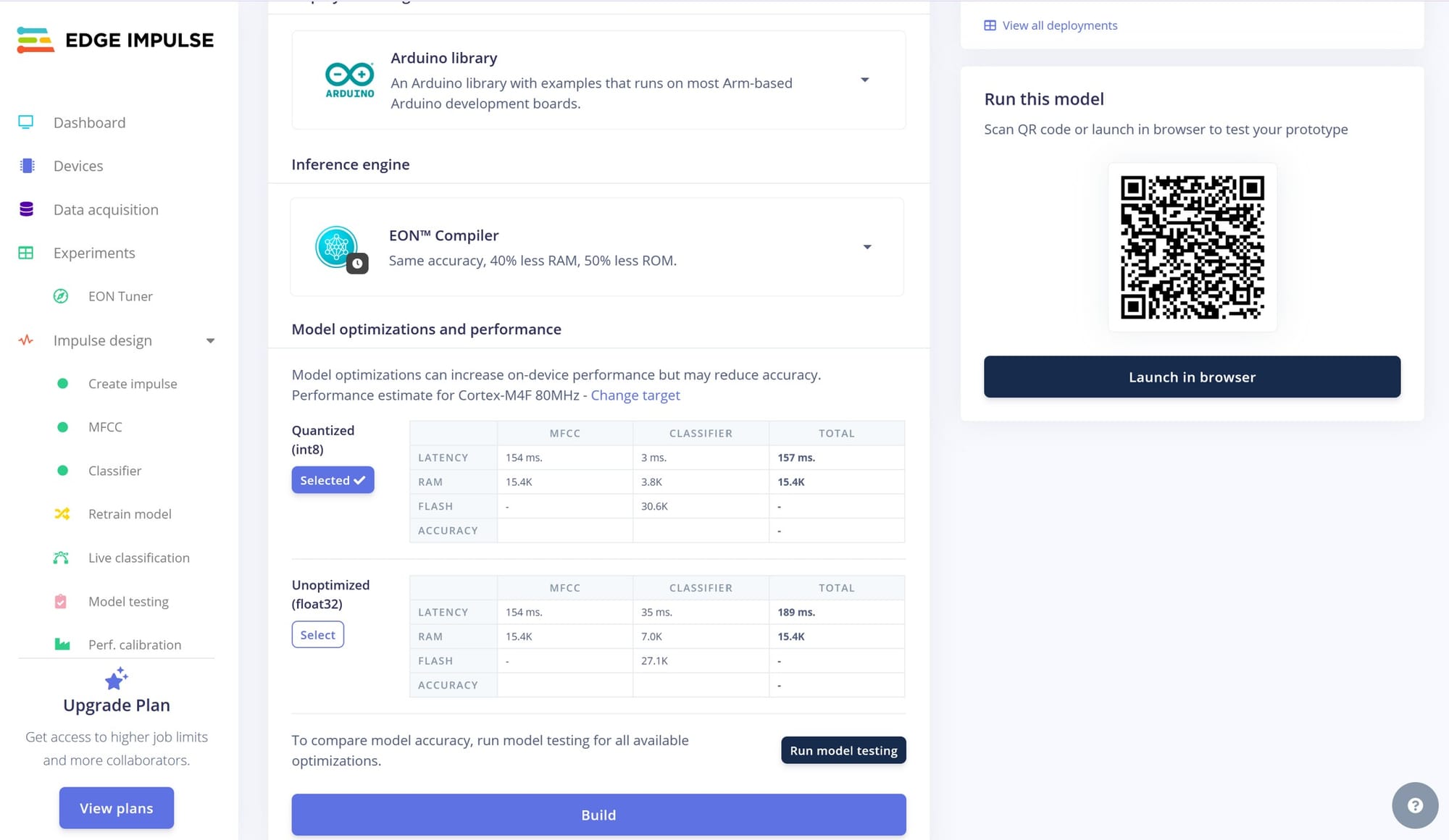
I timed the classifier on the ESP32-S3: 3 ms for INT8 and 35 ms for floating point. Three milliseconds felt quick, but the feature-processing stage still needed attention. I kept its timing separate from the classifier so I could see where the complete processing pass spent its time.
The rest of the table makes the comparison more interesting. MFCC took 154 ms in both versions, so the totals are 157 ms and 189 ms. The classifier stage changes much more than the complete processing time. That gives me a useful way to think about optimisation: the most attractive number can describe only one part of the work, while the audio representation, memory requirements and other stages still belong to the application.
That doesn't make the screen useless. I can still compare the options it shows under its assumptions. The table contrasts INT8 and floating-point classifier times, including 3 ms and 35 ms. The question is what that comparison helps me understand, and which parts I would still have to measure on the actual device.
INT8 is a clue about representation. Instead of keeping all the relevant model values as floating-point numbers, a quantised model uses a limited integer representation with scaling. That can change storage and computation. It isn't simply removing decimal points from the printed answer, and it doesn't guarantee the same improvement on every processor.
A ruler helps me think about the tradeoff. If I replace a very fine scale with fewer marked positions, I need a way to map the values into those positions and interpret them afterwards. That analogy doesn't describe the entire quantisation process, but it reminds me that range and precision have to be handled. A smaller representation isn't automatically free of effects on predictions.
A very small storage example makes the appeal clearer. One thousand individual 8-bit values take one thousand bytes before any extra information is included. One thousand 32-bit values take four thousand bytes. That’s just arithmetic about representations. It’s not proof that the entire exported application becomes four times smaller, because the program contains other things too.
The processor and software support matter too. Different devices handle different operations differently. The model's size and layer types also affect the work. I can't take a measured speed ratio from one target and multiply a timing from a different board by it. The ratio belongs to the comparison that produced it.
There's a second boundary in the table: classifier work isn't necessarily all the work between receiving sound and producing a useful response. The audio has to be captured and converted into features. The application has to move data and handle results. A short classifier time doesn't make those stages disappear.
This is familiar from the converter efficiency figures. The number is most useful when I keep the conditions around it. Here, the conditions include the target, clock assumption, representation and scope of timing. It’s the same kind of mistake to crop them away and carry only the largest saving into a sentence about the project.
Memory needs a similarly careful reading. Flash storage for the program and model is different from working memory needed while things run. I want the actual table and exported build information, with labels saying what each value covers.
A model can fit in storage while the complete application still needs attention. There are audio buffers and processing requirements around it. I don't want to count only the model file, call that the device's memory use and then wonder why the application has a different requirement. The code doing the useful job is larger than one attractive number on a deployment page.
The thing I want to ask my mentor is how to arrange a fair comparison on the actual target. Same input, clear versions, same timing boundaries and enough repeated runs to understand the behaviour.
I also want prediction quality kept beside performance. If one representation produces different decisions, the timing comparison needs that information. A faster classifier may still be useful, but speed and correctness answer different questions. I can't prove the second by showing the first.
The exported model and the application code need to stay together in the notes. If I later change the model but keep an old timing capture, the result could quietly become attached to a version that never produced it. It’s easier to preserve the link now than reconstruct it from screenshots later.
For today, the practical correction is small. Three milliseconds stays on the deployment screenshot with ESP32-S3 and timing beside it. The actual board gets its own open timing question. I can still be interested in the improvement without pretending it has already happened on our setup.
The memory rows also resist a simple smaller-is-better sentence. Classifier RAM is listed as 7.0K for float and 3.8K for INT8, while classifier flash rises from 27.1K to 30.6K. The listed total RAM stays at 15.4K. Those are more useful details than applying the general EON banner's saving percentages to the whole application. The export does use a compiled INT8 model, but the consequences need to be read by category and kept attached to the stated target and table.
Reading the target name has made deployment more interesting rather than less. The model is becoming software that has to run on particular hardware, with particular instructions and memory. That's exactly the connection I wanted to understand when I started putting the microphone and the board together.